AP Calculus Study Guide: Key Formulas and When to Use Them
This AP Calculus study guide helps you choose a formula for the quantity a problem asks for and check when that formula is valid. Start with the shared AB core, adding the marked BC tools if you take BC. Reconstruct the connected examples, then close the guide and solve a new problem. Use it for understanding and method selection; it is neither a complete syllabus nor a practice exam.
Match the reference to your AB or BC course
AP Calculus AB and BC share limits, derivatives, and integral calculus. The official course outline organizes AB into eight content units. BC includes that content, adds material inside several shared units, and has additional units on curves and infinite series.
| Content area | Shared AB and BC work | Additional BC work |
|---|---|---|
| Units 1–3: limits and differentiation | Limits, continuity, derivative definition, differentiation rules, implicit and inverse derivatives | The shared foundation remains necessary |
| Units 4–5: derivative applications | Motion, related rates, linearization, L’Hôpital’s rule, extrema, concavity, optimization | The shared foundation remains necessary |
| Unit 6: integration | Riemann sums, accumulation, FTC, antiderivatives, substitution | Integration by parts, linear partial fractions, improper integrals |
| Unit 7: differential equations | Slope fields, separation, initial conditions, exponential models | Euler’s method and logistic models |
| Unit 8: integration applications | Average value, motion, area, cross sections, disks and washers | Arc length and distance along smooth planar curves |
| Units 9–10 | Not AB content units | Parametric, polar, vector-valued functions; sequences, series, Taylor and Maclaurin work |
The formulas developed here connect selected parts of those areas. You will still need separate practice in related rates, optimization, slope-field drawing, numerical integration, and further series tests; this reference does not teach every listed skill. Use your course syllabus and the official outline to identify unfinished topics. If your task is choosing a course, start with the AB vs BC guide.
College Board states that course content has not changed for 2026–27, while multiple-choice question counts and timing change starting with the May 2027 exams. Check the current exam page before doing exam-paced practice. A knowledge reference does not establish a practice-exam schedule or predict a score.
The AB core: definitions and derivative rules
Limits, continuity, and the derivative
At an interior point, a finite two-sided limit exists when the left- and right-hand limits exist and agree. Continuity additionally requires the function to be defined there and to take that limiting value:
To find an instantaneous rate, take a derivative. An ordinary ratio of function values does not give that rate. MIT’s calculus syllabus describes derivatives as limits of ratios and integrals as limits of Riemann sums. The derivative definition is
when this limit exists as a finite number. If measures meters and its input measures seconds, the derivative measures meters per second. A finite-interval difference quotient measures an average rate. Taking its limit gives the instantaneous rate.
Continuity alone is insufficient. For , the function is continuous at , but the difference quotient there is . It equals for and for , so there is no finite common derivative. This distinction matters when a theorem requires differentiability: an unbroken graph can still have a corner.
Choose rules from the expression’s structure
Read the expression’s structure first: sum, product, quotient, composition, or implicit relation. You may need several rules in one calculation. The chain rule requires the inner function to be differentiable at the input and the outer function to be differentiable at the inner output.
In this table, and are differentiable wherever the formula is used. Trigonometric inputs are in radians; the trigonometric derivatives apply on each function’s domain. OpenStax’s differentiation rules supply the algebraic rules, and its exponential–logarithmic derivatives supply those two function families.
| Form | Derivative | Condition or check |
|---|---|---|
| ; | ; | and are constants; use the power rule on the real domain where the function is differentiable, not automatically at an endpoint |
| ; | ; | The logarithm requires |
| ; | ; | Keep the inner derivative |
| ; | ; | Require |
| ; | ; | Require |
| ; | ; | For the displayed arcsine derivative, require |
| ; | ; | A product does not differentiate into |
| Require | ||
| Evaluate the outer derivative at , not at |
For example, differentiate . Both factors are differentiable for all real . Apply the product rule, then the chain rule to the exponential:
Factoring gives . Check what each term accounts for. The first comes from differentiating the polynomial, the second from differentiating the exponential. Missing the factor means the inner rate was lost.
For an inverse, the derivative is evaluated at the original input corresponding to the inverse’s argument. If has a differentiable inverse locally and , then
The inverse-function reference explains this inverse-image condition. Check global invertibility separately; the table does not establish it.
For an implicit relation, follow the implicit-differentiation strategy along a differentiable solution branch, treating as a function of . For example, gives , so where . If the divisor is zero, investigate the point rather than dividing. For local linearization at a differentiable input , use ; this is a nearby approximation, not an identity for every .
Keep the hypothesis beside the theorem
Check a theorem’s hypotheses before using its conclusion. College Board’s clarifications explicitly retain a closed interval in the extreme value theorem. A formula list that keeps only the conclusion leaves out a necessary hypothesis.
| Tool | Check before using it | What it establishes |
|---|---|---|
| Intermediate value theorem (IVT) | continuous on | Every value between and is attained somewhere in ; it does not guarantee uniqueness |
| Extreme value theorem (EVT) | continuous on the closed, bounded interval | Absolute maximum and minimum values are attained |
| Mean value theorem (MVT) | continuous on , differentiable on , and | Some satisfies |
| L’Hôpital’s rule | Quotient has form or ; numerator and denominator differentiable in a punctured neighborhood, with both the denominator and its derivative nonzero there, and the derivative quotient has the required limit | Under these hypotheses, the quotient limit agrees with the derivative-quotient limit; handle one-sided limits consistently |
The continuity reference states the IVT and distinguishes continuity from merely having endpoint values. The MVT reference makes the secant–tangent relationship explicit. In this separate example, the hypotheses hold and the slopes match.
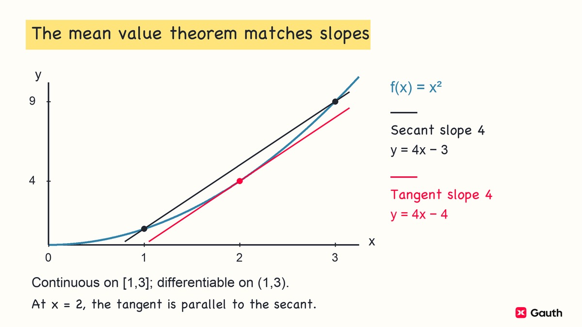
For on , the secant slope is , but the derivative is never where it exists. The missing differentiability at prevents the MVT guarantee. For on , continuity does not supply an attained maximum: the interval omits its upper endpoint. Without a hypothesis, the theorem no longer guarantees the conclusion. That does not mean the conclusion must be false in every such case.
For a continuous closed-interval extrema problem, compare function values at endpoints and interior critical numbers, where or does not exist. The extrema reference distinguishes candidates from confirmed extrema. For local extrema, examine the derivative’s sign change. For inflection points, examine a change in concavity; by itself is only a candidate condition.
Check the quotient’s original limiting form before applying L’Hôpital. The L’Hôpital reference cautions against applying the rule to a quotient that is not indeterminate. For as , the numerator approaches , not . Differentiating the numerator and denominator would incorrectly suggest a finite answer. The right-hand limit is and the left-hand limit is .
From rates to accumulated change
The FTC and substitution reverse the chain rule
For continuous on , define . The fundamental theorem of calculus gives at interior inputs. If , its other standard form gives
Use the first statement to differentiate an accumulation function and the second to evaluate a definite integral from an antiderivative. In either case, keep the conditions and distinguish a signed integral from geometric area.
For differentiable bounds and , with continuous on the relevant integration intervals,
Take . The polynomial integrand is continuous, so
Account for both moving bounds. The lower bound contributes the subtracted term, which disappears if you differentiate only the upper bound.
Substitution uses the same chain rule in reverse. For , write and transform every part of the integral. The substitution reference also changes the bounds in a definite integral:
with continuous and continuous on the needed range. Monotonicity of is not required for this identity, although geometry may require you to separate retraced pieces.
For , set and . The bounds become and , and :
A corresponding antiderivative is . Differentiating it returns the original integrand and checks the antiderivative. To check the definite value, verify the transformed limits as well.
One motion model, several different questions
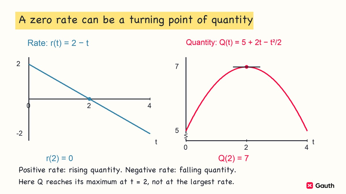
MIT’s integral unit connects a known rate and an initial value to the value of a quantity. The net-change theorem expresses that connection as
when the rate is continuous. The graph of gives the slopes of , rather than the heights of . The illustration uses a separate model to keep the two functions distinct.
Now consider an original one-dimensional motion model, with position in meters and time in seconds:
Find its velocity, acceleration, intervals of increasing speed, displacement, total distance, and average rates. All quantities must be interpreted on the given interval.
Differentiation gives
The velocity is positive on , negative on , and positive on . Thus the particle reverses direction at and . At , acceleration is zero while velocity is ; zero acceleration does not mean the particle has stopped.
For nonzero velocity, speed increases when and have the same sign. Here it increases on and , and decreases on and . Negative velocity with negative acceleration means motion in the negative direction is becoming faster.
Evaluate the position at the endpoints and turning inputs:
| (seconds) | ||||
|---|---|---|---|---|
| (meters) |
The absolute minimum position is meters, attained at and ; the absolute maximum is meters, attained at and . These are position extrema, not statements about maximum speed.
Displacement is signed change:
Total distance adds the magnitudes of the three movements:
For displacement, subtract the backward movement from the forward movements. For distance, add all three movement lengths: forward, backward, and forward.
Average velocity is meter per second. Average speed is meters per second. More generally, the average value of continuous on , with , is
Use for average velocity and for average speed. Choose the integrand from the quantity you need to measure.
Initial-value problems and geometric accumulation
A differential equation gives the rate relation. Its initial condition selects the required solution from the possible solutions. For with , first note the equilibrium solution . It does not satisfy the given initial condition. On a nonzero branch, separation gives
The general family is , and the initial condition gives . Verify twice: differentiation gives , and substitution gives . The separation strategy checks constant solutions before division, so it does not silently exclude them.
Geometric accumulation begins by identifying the cross-sectional quantity. The slicing reference integrates cross-sectional area, rather than a side length. If a solid has continuous cross-sectional area , then . For a region bounded by and on , suppose sections perpendicular to the -axis are squares. Their side length is , so
The area has squared length units and the volume has cubed length units. Integrating the side length instead would calculate a planar area, not the volume of the square-section solid.
For washers, use , where the radii are nonnegative distances from the rotation axis and . A region crossing the axis may require a disk or a split setup. For planar area between graphs, integrate over the specified interval, splitting at intersections as needed; a signed difference without checking which curve is above can cancel genuine area.
BC additions: curves, convergence, and approximation
BC students need the AB core as well as these added tools. For a broader college-course orientation, use the Calculus 2 guide, but do not treat every Calculus 2 topic as an AP BC requirement. The official AP outline, rather than a college textbook’s chapter list, defines that boundary.
Extra integration and differential-equation tools
For functions with continuous derivatives, integration by parts reverses the product rule:
Choose so its derivative helps, and choose so it can be integrated. Keep the remaining integral when writing the answer. For linear partial fractions, factor the denominator, perform polynomial division first if the fraction is improper, then solve the coefficient identity. For example,
Check the decomposition by adding the fractions on the right. Integration gives on intervals avoiding those excluded inputs.
An infinite limit or a singular integrand makes an integral improper. Replace the offending bound with a limit; if there are separate singular pieces, each must converge. For example,
Evaluate finite integrals first, then take their limit. Infinity is not an ordinary real input to substitute.
For , Euler’s method with step uses
Each step uses the slope at the current approximate point. It gives an approximation, and its error depends on the equation, step size, and interval; do not label it an exact solution. The logistic model is with constant and carrying capacity . Its equilibrium populations are and ; the derivative is positive for and negative for . Check these signs before interpreting a modeled population change.
Parametric, vector, and polar formulas
For a twice continuously differentiable parametric curve , , the parametric-calculus reference gives, where ,
For the second derivative, differentiate with respect to again. It is not .
For , , with ,
At , the slope is and the second derivative is . Eliminate the parameter locally to check: gives the same derivatives at .
For a twice continuously differentiable vector position , the vector-motion definitions differentiate each component to obtain velocity and again to obtain acceleration. Speed is . Integrating speed gives the path length traveled; displacement is the difference of position vectors. If a parametrization retraces part of a curve, its speed integral counts that traversal again. For a graph with continuous derivative, the arc-length formula is .
In polar coordinates, write and . For differentiable , applying the product rule to these two coordinates and dividing their derivatives gives the slope
where the denominator is nonzero. The polar-area reference derives area from sectors:
Use radians and an interval that describes the intended region without counting it repeatedly. In the basic sector setup, is continuous and nonnegative and . For on , the region is a quarter disk and . Between two nonnegative polar radii on the same angular interval, subtract the inner squared radius from the outer squared radius; first determine which one is outer.
Series tests, endpoints, and Taylor bounds
A series is the limit of its partial sums, when that finite limit exists. Terms approaching zero are necessary but not sufficient for convergence. The harmonic series is a familiar counterexample.
| Situation | Useful first test | Limit of the conclusion |
|---|---|---|
| The term does not approach zero | Nth-term divergence test | A zero term limit is inconclusive |
| Constant term ratio | Geometric series | Converges for ; do not extend its sum formula outside that range |
| Factorials or powers simplify in a term ratio | Ratio test on absolute values | Limit below gives absolute convergence, above gives divergence, and is inconclusive |
| Alternating signs | Alternating-series test | Positive term magnitudes must decrease eventually to zero; this alone does not establish absolute convergence |
The ratio-test reference uses nonzero terms and an existing absolute-ratio limit. The alternating-series reference supplies the decreasing-to-zero condition and omitted-term error bound. This selection covers the examples here, not every test in BC. Integral, comparison, and -series tests remain part of the official course scope.
For a power series, determine its interior convergence first, then check each endpoint independently. The power-series theorem permits different endpoint behavior even when the radius is known.
Consider
It is geometric with ratio . It converges for , giving radius and interior . At , the terms are ; at , the terms are . Neither sequence of terms tends to zero, so both endpoints are excluded. Within the interval,
At the center , interpret the zeroth term as . Use the sum formula only within the series’ convergence interval.
Taylor approximation also needs a separate validity check. For a function sufficiently differentiable near , the order- Taylor polynomial is
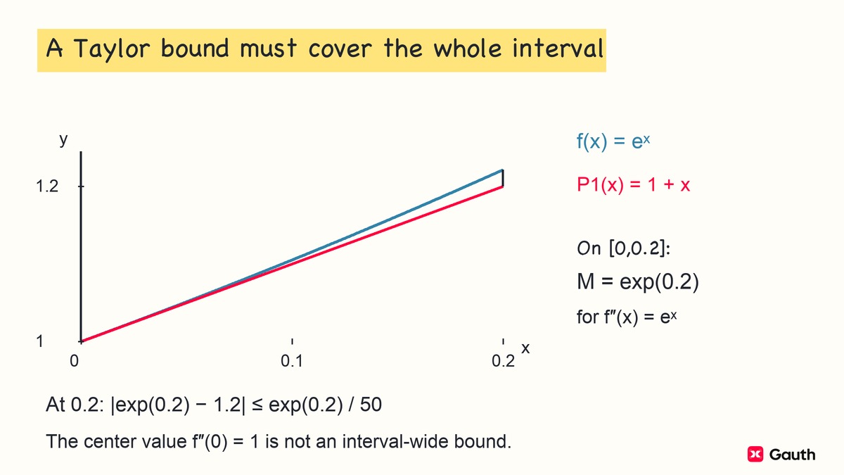
Maclaurin means . The finite polynomial alone does not show that the infinite Taylor series equals the function. For a remainder bound, Taylor’s theorem requires derivatives through order on the interval between the center and the evaluation input. If throughout that interval, then
The illustration uses a separate exponential example to distinguish the derivative value at the center from an interval-wide bound.
For , the order-three Maclaurin truncation is , because the linear and cubic coefficients vanish. Its actual degree is two; retaining the order-three interpretation lets you apply the remainder theorem with the fourth derivative. At ,
The fourth derivative is , whose absolute value is at most on . Therefore
This estimates an upper bound, not the actual error. Match the derivative order to the truncation, then justify throughout the interval. A derivative value at the center is insufficient.
For an alternating-series approximation meeting the decreasing-to-zero conditions, the error is at most the magnitude of the first omitted term. That is a different justification from the derivative-based Taylor bound; state which one supports your answer.
Use the reference, then solve without it
Choose one connection you cannot yet explain. A possible -minute session allocates minutes to definitions and conditions, to reconstructing one worked example, and to an unfamiliar problem without the reference. These times are an adjustable example, not an experimentally established optimum or an AP pacing rule.
Before trusting your answer, ask what each symbol represents, whether the required domain and hypotheses hold, and how to check the result. Differentiate an antiderivative, substitute a proposed solution into both a differential equation and its initial condition, or compare a numerical result with the signs and units in the model. You still need to check the theorem’s hypotheses, even if a calculator gives an answer.
If a formula is entirely new, return to your teacher’s explanation or course materials before mixed review. If you can reconstruct the example, change its data: use a different initial position in the motion model, or change one integral bound. The derivative stays unchanged when a constant is added to position, while the position values change. Explain that relationship before calculating again.
Once the conditions and method are familiar, attempt mixed AP Calculus review questions with answers hidden, including both calculator and no-calculator work from your assigned materials. This reference remains available for checking a specific gap; it does not replace those attempts or official scoring guidance.
For optional guided practice, open Create Course and enter your AP AB or BC level with one specific topic, such as “choosing between net change and total distance.” Use the generated course as learning support, check mathematical steps against your course materials or teacher, and follow your school’s AI guidance. It does not certify complete AP coverage or validate a predicted score.
Sources and review
Sources checked November 10, 2026. Examples in this guide were written for the article; they are not released College Board questions. Textbook references support the specified definitions, formulas, and hypotheses, not an endorsement of the whole guide.
- Official course outline: shared content and BC additions.
- Current exam page: course-content clarification and exam updates effective May 2027.
- MIT’s calculus syllabus: derivative and integral definitions; the MIT syllabus is not the AP scope.
- College Board’s clarifications: closed-interval EVT statement and differential-equation clarification.

