Inferential Statistics: From a Sample to a Conclusion
Inferential statistics uses sample data and probability models to estimate population quantities or test hypotheses about them. Its conclusions depend on the sampling design and the method's assumptions, not just correct arithmetic. Define the population, check how the data were collected, and report the estimate with its uncertainty. A confidence interval and a p-value answer different questions; neither proves that a sample represents everyone or that an observed association is causal.
What makes a conclusion inferential?
A conclusion becomes inferential when it reaches beyond the observations. JMP's statistics introduction describes statistical inference as drawing conclusions about a population from sample evidence, using probability theory to quantify uncertainty. Estimating a population mean, testing a claim about that mean, and estimating a relationship through a statistical model are examples of inferential tasks.
A population is the collection of people, objects, events, or measurements your question concerns. A sample contains the observations collected from it. A parameter, such as a population mean, describes the population; a statistic, such as a sample mean, is calculated from the observed sample.
Descriptive and inferential statistics can begin with the same numbers. Reporting the mean time among the participants you measured is descriptive. Using those participants to estimate a mean for a specified larger population is inferential. To make the second claim, explain the sampling or modeling basis and quantify its uncertainty.
If you need help calculating a mean or sample standard deviation, work through descriptive statistics first. Here, we use those summaries to examine claims beyond the sample. Keep the original observations available for checking.
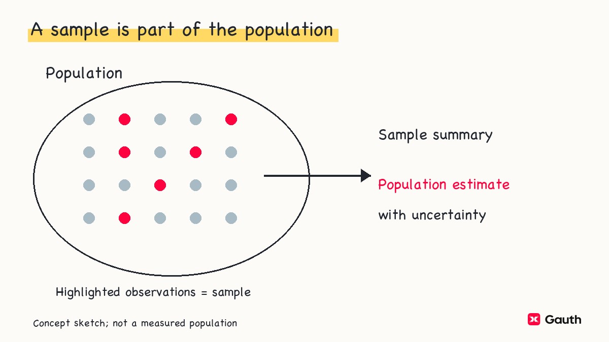
The highlighted points below are part of the larger collection, not a separate population. Summarizing them is one action; making a claim about the larger collection requires additional reasoning.
Check the sample before choosing a formula
Begin by writing the population and the quantity you want to estimate. “Students” is often too broad: the target might be students enrolled at a particular college during a specified term. A sample from one class does not automatically represent that college, and a college sample does not automatically represent all students.
JMP explains why the sampling plan limits the population to which you can make inferences. Simple random sampling gives every possible sample of the chosen size an equal selection probability. It supports a probability-based account of sampling variation, but it does not guarantee that every realized sample matches every characteristic of the population.
Convenience sampling can systematically favor the observations easiest to obtain. For example, asking only people already using a study room can underrepresent students who do not use it. A larger sample from that same selection process may retain the bias. A narrow interval from a simple sampling model leaves other possible selection and measurement errors unmeasured.
Check what one row represents. Repeated measurements on the same person, observations from the same household, and time-ordered measurements can have dependence that a simple independent-observation formula ignores. Do not count repeated readings as separate independent people merely because they occupy separate rows.
Also distinguish random selection from random assignment. Selection concerns who or what enters the sample. Assignment concerns which treatment an enrolled participant receives. A well-designed controlled experiment can support a causal question; a random sample alone does not turn an observational association into a treatment effect. JMP distinguishes these study-design responsibilities.
Before proceeding, identify the response variable, units, missing observations, selection process, and potential dependence. If any of those changes the question or method, resolve it before interpreting the software output. Software can return a precise number for a question your data cannot answer.
A worked inferential statistics example
Suppose a teaching problem gives this summary of task-completion times, in minutes:
Here, is the sample size, is the sample mean, and is the sample standard deviation. The question concerns the population mean completion time, , and a fixed benchmark of minutes.
These are invented summary inputs, not a real student study. For this calculation, stipulate independent observations drawn from the target population and a normal population model with unknown population standard deviation. These assumptions define the teaching problem; they have not been established by inspecting raw records. In an actual analysis, the summary alone would not let you check outliers, shape, selection, or dependence.
We will estimate the mean and then perform a two-sided test of whether it differs from the benchmark. Choose that question and the significance level before examining the result.
Turn the sample summary into a standard error
Standard deviation measures spread among observations. The standard error of the mean concerns how sample means vary across repeated samples under the model. Although both measures have the same units, they describe different sources of variation. Penn State's one-sample lesson uses the sample standard deviation to estimate the standard error when the population standard deviation is unknown:
Substitute the stipulated summary:
The observed times have a sample standard deviation of minutes; the estimated standard error of their mean is minute. This does not say that individual completion times are within minute of the mean.
In the independent, identically distributed setting, increasing sample size reduces the theoretical standard error for a fixed population standard deviation. It does not remove selection bias, make measurements independent, or guarantee that the observed sample standard deviation stays unchanged.
For this one-mean calculation with unknown population standard deviation, use a t distribution with:
The t distribution accounts for estimating the population standard deviation. Sample size alone does not decide whether to use t or z. In particular, reaching observations is not a universal instruction to switch to a z-test. The population model, known versus estimated standard deviation, and sampling design matter.
Estimate the population mean with a confidence interval
A point estimate assigns a single value to the unknown population quantity. Here, the point estimate of is minutes. An interval shows the uncertainty associated with the chosen estimation method.
NIST's mean interval uses the t quantile, sample standard deviation, and sample size. For a two-sided confidence level of , the formula is:
For a interval, . The required t quantile has cumulative probability and degrees of freedom:
Multiply this value by the estimated standard error to find the margin of error, then subtract and add it:
Under the stipulated model, the interval is an estimate of the population mean, not a range containing of individual completion times. It also does not mean that the fixed population mean has a probability of lying inside this particular calculated interval.
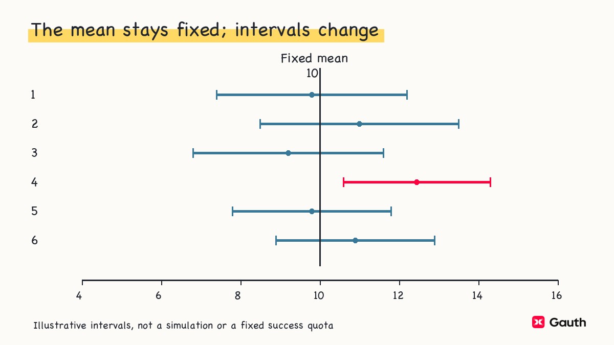
NIST attaches the confidence level to the procedure: if we repeatedly sampled and constructed intervals in the same way, approximately would contain the fixed population mean in the long run, assuming the method's conditions hold. The interval endpoints change across samples; the parameter does not.
The following small illustration shows intervals crossing or missing one fixed mean. It is not a simulation result and does not require any fixed fraction of a small batch to succeed.
Keep the unrounded quantile during calculation and round the final endpoints for reporting. If a calculator differs, check the confidence level, degrees of freedom, sample versus population standard deviation, and whether it is producing a mean interval or an interval for individual predictions.
Test a benchmark mean with a two-sided t-test
The interval asks how precisely we have estimated the mean. A hypothesis test asks how incompatible the observations are with a specified null model. For the benchmark question, write:
Both hypotheses are statements about the population mean. The observed sample mean has already been calculated; its equality to the benchmark is not what the test asks. The alternative is two-sided because departures in either direction address the chosen question.
Using the same conditions and estimated standard error, calculate:
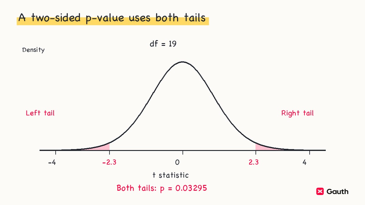
The statistic is negative because the estimate falls below the benchmark. For the two-sided p-value, use the t distribution with degrees of freedom and include both tails at least as far from zero as the observed statistic:
Under the null and the model's assumptions, this is the probability of obtaining a t statistic at least as extreme in the chosen two-sided sense. It is not the probability that the null hypothesis is true or the probability that the result was caused by chance alone. The ASA's p-value principles explicitly reject those interpretations.
With the preselected , the p-value is larger than the threshold, so fail to reject the null hypothesis. This test provides insufficient evidence of a difference at the selected level. Do not replace that statement with “the population mean is exactly minutes.”
As a consistency check, the matching two-sided t interval contains . NIST explains the relationship between the two-sided interval and test using the same model and significance level. An interval for a different parameter, a different confidence level, or a one-sided question is not the same check.
This separate t curve illustrates the two-tail operation with a different statistic and degrees of freedom. Both shaded regions contribute to its p-value.
Choose a method for a different question
Inferential statistics is broader than one t-test. JMP groups inferential work into interval estimation, hypothesis testing, and fitting statistical models. Choose the quantity and design first, then a method that answers that question.
| Your question | Inferential target | What changes from the worked example |
|---|---|---|
| What is a population's average numerical response? | A population mean | Check the sampling model, independence, spread, and mean-interval conditions |
| What fraction of a population has a defined outcome? | A population proportion | Use counts and the denominator; a mean-time t interval is not a proportion interval |
| Do defined groups differ? | A contrast between population quantities | Identify independent groups or linked observations; use a method for that contrast |
| How does an outcome relate to specified predictors? | Parameters or predictions from a statistical model | Define the model and check its assumptions; a fitted association alone does not establish causation |
An analysis can report both descriptive summaries and inferential results. A fitted line may summarize the observations; using its parameters or predictions beyond those observations adds inferential questions. Identify the quantity attached to each reported uncertainty measure.
Penn State’s ANOVA lesson treats analysis of variance as a test of hypotheses about group means. Its name does not mean that any comparison of observed variances answers the group-mean question. This guide does not provide a complete ANOVA procedure or a universal test-selection chart.
The one-sample t formula above is not suitable for every numerical data set. Different sampling designs, severe departures from the population model, or a different target quantity can require another analysis. Some alternatives use resampling or ranks, but “nonparametric” does not mean “assumption-free,” and a small sample alone does not select an alternative. Consult the method's conditions and the assignment's requirements.
What significance and non-significance do not prove
A significant result is not automatically important. The ASA distinguishes a p-value from effect size and practical importance. A very precisely estimated small departure can produce a small p-value; deciding whether that departure matters requires the estimate, uncertainty, context, and a relevant criterion.
A non-significant result does not establish equality or absence of an effect. In our example, the interval allows means below the benchmark as well as the benchmark itself. The test has not narrowed the uncertainty enough to justify every possible claim about the difference.
Likewise, do not use a p-value to judge sample quality. Correctly applying a test to a convenient sample does not give the excluded population members a chance of entering that sample. Report the selection limits separately from the test result.
Avoid changing the question after seeing the answer. Choosing a favorable tail, trying many outcomes and reporting only the smallest p-value, or dropping observations without documenting the reason can make a result misleading. The ASA emphasizes full reporting and transparency. Explain the analysis choices and relevant changes, including results that do not pass a selected threshold.
Keep causal claims tied to design. A difference between two observed groups might reflect other differences between those groups. A small p-value does not identify which explanation produced the association.
Report the estimate, uncertainty and limits together
For the stipulated teaching example, a suitable report is:
Under the independent normal-population assumptions in this example, the estimated population mean completion time was 18 minutes, with a 95% t confidence interval of 15.94 to 20.06 minutes. A two-sided one-sample t-test against 20 minutes gave t(24) = -2 and p = 0.05694. At the preselected significance level of 0.05, we failed to reject the null hypothesis. These invented summary inputs do not establish a causal effect or support generalization beyond the stipulated population.
The report identifies the estimate and units, gives the interval and test results, and states the decision rule and scope. In a real report, identify the population, sampling period, usable count, collection method, missing-data handling, and reasons for any exclusions. Do not copy the teaching assumptions as if you had verified them in your study.
Use software to check the arithmetic while retaining responsibility for the question. Confirm that its selected procedure is the one-sample mean test, the alternative is two-sided, the benchmark is , the degrees of freedom are , and the input spread is a sample standard deviation. If the procedure requires raw data, a mean and standard deviation are not a substitute for those records.
Read the final sentence against the calculation and look for claims it cannot support. Replace “proved equal” with the actual non-rejection decision. Replace “caused” with an association description unless the design supports the causal claim. If the selection process cannot support the stated population, narrow the scope or obtain an appropriate sample before presenting that broader inference.
Practice the part of inference you cannot yet explain
For another numerical-mean problem, first state the target population and parameter. Explain why the standard error differs from the data's standard deviation, construct the appropriate interval, and interpret its confidence level without referring to individual observations.
Then state the null and alternative before calculating a test result. Check that the interval and test refer to the same parameter and compatible levels. Write a report that remains accurate whether the result is significant or non-significant.
If the calculation is correct but your report says “there is a probability that the mean is here” or “the large p-value proves no difference,” practice interpretation before adding more tests. If the sample design is the difficulty, return to defining the population and selection process rather than recalculating the same p-value.
For focused study, open Gauth's Create Course and enter your level and a precise topic, such as introductory inferential statistics, interpreting confidence intervals, or one-sample t-test conclusions. Check the resulting material against the method and assumptions required by your course.
Sources and review
Sources accessed November 10, 2026. The summary inputs and figure examples are illustrative, not records of real students or a measured intervention.
- JMP — Inferential statistics: populations, samples, study design, sampling plans, estimation, testing, and model fitting.
- Penn State — Inference for one sample: the one-mean standard error, t distribution, degrees of freedom, confidence intervals, and hypothesis-test calculations. Relevant one-mean sections were consulted; course-specific sample-size conventions are not universal rules.
- NIST — Confidence limits for the mean: t interval, repeated-sampling interpretation, and the matching two-sided test.
ASA — Statistical significance and p-values: the association's March 7, 2016 release presenting six principles on interpretation, practical importance, and transparent reporting.

