Descriptive Statistics: How to Summarize Data Correctly
Descriptive statistics organize and summarize the data you observed using counts, measures of center and spread, and graphs. Choose summaries that fit the variable and the distribution, then report the number of observations, units, and scope. A sample summary describes that sample; it does not, by itself, justify a conclusion about a larger population. Start with the data type before choosing a formula.
What descriptive statistics can tell you
Use a descriptive statistic to answer a question about the observations you have: which response was most common, how long a typical wait was, or how much the measurements varied. OpenStax's statistics introduction distinguishes organizing and summarizing data from using formal inferential methods to draw conclusions beyond the observed data.
For example, a mean calculated from a classroom survey describes the surveyed students. Estimating the mean for all students at the school is a separate task that depends on how the sample was selected and how uncertainty is handled. Correct arithmetic alone cannot support that larger conclusion.
Descriptive statistics can summarize either a sample or a fully observed population. The word descriptive refers to what you do with the data, not whether the data came from a sample. It also includes tables and graphs, so the subject is broader than calculating an average.
Build the summary around what was measured, its center and spread, and patterns that a few numbers might hide. Select the statistics that answer your question; calculating every available measure rarely makes the purpose clearer. If you need the broader definition first, start with what statistics means.
Choose summaries that fit your data
Identify what each observation represents before choosing a calculation. Interpret a category differently from an ordered rating or a measurement. Curtin's descriptive statistics guide organizes summaries around the variable type and the number of variables being examined.
| Data you have | Useful starting summaries | What to check |
|---|---|---|
| Unordered categories, such as a chosen travel method | Counts, proportions, mode, bar chart | Categories are defined consistently; the denominator is stated |
| Ordered categories, such as low, medium, high | Counts and percentages in order; a middle category when useful | An order does not establish equal numerical spacing |
| Numerical counts or measurements | Mean or median, a spread measure, and a plot | Units, extreme values, distribution shape, and sample versus population |
| Paired numerical measurements | A scatterplot and summaries of each variable | Keep each pair together; an association does not establish a cause |
Suppose six invented responses contain three bus choices, two walking choices, and one bicycle choice. Bus has a relative frequency of , or . This is a description of those responses. If the categories were coded as , , and , the mean of those codes would not be a meaningful average travel method.
Before calculating, check the observational unit: one person, one trial, or one recorded event. Repeated readings from one person are not automatically readings from different people. Retain the original records and use them to check the count.
Missing is different from zero. A blank waiting-time entry does not mean someone waited zero minutes. State how missing entries were handled and how many usable observations remain. Resolve inconsistent units and investigate suspicious values before interpreting the calculator's output.
A worked descriptive statistics example
Suppose you recorded the following six waiting times, in minutes:
These are invented teaching data, not observations from a real service or student study. We will first treat them as a sample and calculate an unweighted summary. Each recorded wait contributes once. Keeping the ordered observations visible makes the middle positions and repeated value easy to check.
Mean, median and mode
These three measures answer different questions about the center or a common value. NIST's location measures define the mean as the sum divided by the count, the median through the ordered middle position, and the mode through frequency.
For the sample mean, add the waits and divide by the sample size:
The mean wait is minutes. It uses every recorded value, and it need not match a wait that actually occurred.
For the median, first sort the observations. With an even count, average the two middle numerical values. Here, those are the third and fourth values:
The median wait is minutes. For an odd count of numerical observations, use the single middle value instead. Sort first; a value in the middle of the recording order may not occupy the middle position in the ordered data.
The mode is minutes because it appears more often than any other wait. A data set can have multiple equally frequent modes. When all values occur equally often, there is no uniquely most common value; check your course's convention for reporting that case.
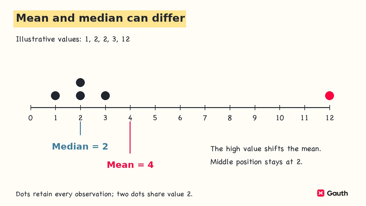
The mean, median, and mode do not have to agree. If the last wait changed from to minutes, the mean would become minutes, while the median would remain and the mode . The middle positions stay the same, but the larger value contributes more to the sum. That does not automatically make the mean wrong: the longer wait may matter to the question being asked.
On the common scale in this separate dot plot, the high value pulls the mean to the right. The repeated low value determines the mode.
Range and interquartile range
A measure of center needs a measure of spread alongside it. NIST's scale measures distinguish measures that use the extremes, the middle portion, or deviations from the mean.
The range is the maximum minus the minimum:
The range is minutes, while the observed waits run from to minutes. Report those endpoints when they matter; the range alone does not tell you where the interval starts.
The interquartile range is the upper quartile minus the lower quartile:
For this hand calculation, use the median-of-halves convention. Split the six ordered waits into the lower half and upper half . Their medians give:
The IQR describes the distance between the quartile cutoffs. It is often paired with the median when the aim is to describe the central portion without giving the extremes as much influence.
Quartiles require a stated convention. An inclusive, linearly interpolated percentile calculation gives and for this same list, so its IQR is minutes. Both results use the same data but a different rule for locating quartiles. Follow the method required by your course or report, and name it when comparing software with hand work.
Sample variance and standard deviation
Variance summarizes squared deviations from the mean. Standard deviation is its square root, restoring the original units. OpenStax's spread chapter distinguishes sample and population formulas. Use the sample formula when these observations are being treated as a sample from a larger population.
For a sample with more than one observation:
The mean is minutes. Subtract it from each wait, then square each deviation.
| Wait (minutes) | Deviation (minutes) | Squared deviation (minutes squared) |
|---|---|---|
| 2 | -4 | 16 |
| 4 | -2 | 4 |
| 4 | -2 | 4 |
| 6 | 0 | 0 |
| 8 | 2 | 4 |
| 12 | 6 | 36 |
| Total | 0 | 64 |
The signed deviations sum to zero because the mean balances them. Squaring avoids that cancellation when measuring spread. Divide the squared-deviation total by one less than the sample count:
Then take the square root:
The sample standard deviation is approximately minutes. It measures spread around the mean, but it is not the arithmetic mean of the absolute distances. For these waits, the absolute distances sum to minutes, giving an average absolute deviation of minutes. NIST treats that as a different spread measure.
Define the population before changing the denominator. If the six waits are the entire finite population you want to describe, let its size be and its mean be . The population calculations are:
Decide what population the question defines before choosing the denominator. “All rows in my file” does not necessarily mean “the entire population I want to describe.” A file may contain every recorded observation from a sample.
Check that a reported variance or standard deviation is nonnegative and that the units are correct. Keep unrounded values during calculation, rounding the final report as needed. A larger standard deviation means more spread on a comparable scale; it does not by itself mean the mean is larger.
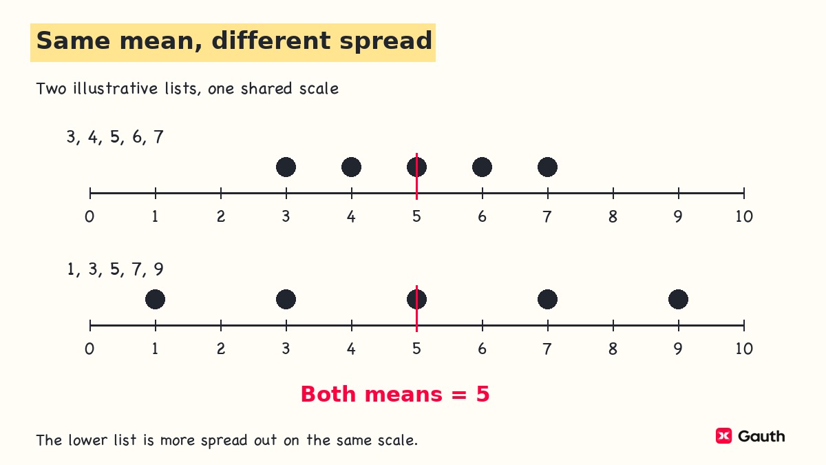
The following two invented lists have the same mean. Their dots show why reporting that mean alone would conceal a difference.
Use a graph to check the summary
Inspect a graph for clusters, gaps, tails, and unusual observations that the numerical summary may miss. For the small waiting-time list, a dot plot keeps every observation visible. Repeated values should appear as stacked dots, not as a single point that hides their frequency.
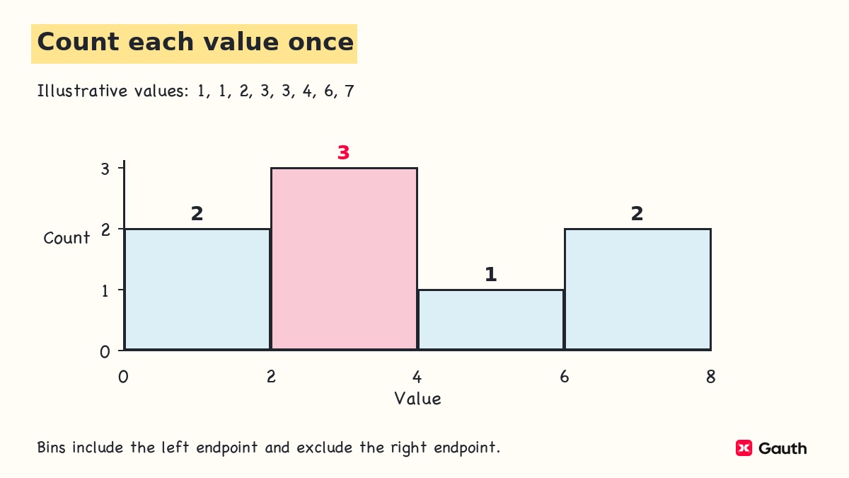
A histogram groups numerical observations into intervals called bins. OpenStax's histogram chapter explains adjoining intervals and consistent boundary rules. Histograms can display discrete numerical data as well as continuous measurements.
For a simple frequency histogram, use equal-width bins and label the horizontal variable and vertical count. Make the boundary convention explicit so each observation enters only one bin. Try another reasonable bin width or starting point. The visible shape can change with the grouping, so one histogram should not settle every question about the distribution.
This example includes the left endpoint and excludes the right endpoint of each bin. A value on a shared boundary belongs to the bin that starts there, and the bar counts add back to the number of observations.
Use a bar chart for unordered categories rather than placing their codes into numerical bins. The order and spacing of category bars do not establish a numerical distance between categories.
A box plot condenses numerical data through the median and quartiles. State the quartile and whisker conventions; whiskers do not always mean minimum and maximum. A box plot does not automatically display the mean. For a small data set, keep the observations or a dot plot available because the condensed display can hide detail.
When you have two numerical variables recorded for the same observational units, a scatterplot displays their paired values. Curtin distinguishes this bivariate task from summarizing one variable. A plotted relationship describes the observed association; establishing a cause or generalizing it requires additional evidence.
Check descriptive statistics in Excel
Use software to check the calculations after confirming that the range and function match the question. For a check of this example, enter only the six numerical waiting times in cells
A2:A7. Keep the unit in the column heading and leave any genuinely missing values distinguishable from zero.Useful checks include
=COUNT(A2:A7), =AVERAGE(A2:A7), =MEDIAN(A2:A7), and =MAX(A2:A7)-MIN(A2:A7). They should agree with the count, mean, median, and range you calculated above. Count the numeric observations before interpreting any other result.For the sample standard deviation, use
=STDEV.S(A2:A7). Microsoft's STDEV.S documentation specifies the sample, one-less-than-count method and directs users to STDEV.P for an entire population. Here, those functions correspond to the sample and population results above. Do not switch functions just to make a result match another answer.For quartiles,
=QUARTILE.INC(A2:A7,1) and =QUARTILE.INC(A2:A7,3) use inclusive percentiles. Microsoft's quartile documentation identifies these as the lower and upper quartiles. The inclusive calculation for this example gives the alternative quartile values discussed earlier, not the median-of-halves upper quartile.If a result differs from hand work, check the data range, whether numbers were stored as text, the number of usable observations, the sample versus population choice, and the quartile convention. These are formula-based checking instructions, not a claim that a particular workbook or Excel interface was tested here.
Write a descriptive report with clear limits
A report should identify the data, summarize relevant features, and state the scope. For the invented sample, a suitable numerical report is:
In the six recorded waits, the mean was 6 minutes and the sample standard deviation was approximately 3.58 minutes. The median was 5 minutes, and waits ranged from 2 to 12 minutes. Using the median-of-halves convention, the lower and upper quartiles were 4 and 8 minutes, giving an IQR of 4 minutes. These summaries describe the six recorded waits.
This report states the count and units and identifies the sample standard deviation, endpoints, and quartile convention. Your assignment may need fewer measures. Explain the choice in relation to its question, rather than copying the full software output.
Investigate an unusually high wait before deciding whether to exclude it. It may record a genuine experience, a different process, or an error. Check the original record and the inclusion rule. If a correction or exclusion is justified, document it and retain the original data rather than quietly changing the summary.
A correct descriptive report does not repair an unrepresentative sample. If only convenient observations were collected, adding more decimal places cannot establish that the results represent everyone else. Keep a population claim separate from a description of the observed sample.
Likewise, a group difference or association can be described without proving a cause. Inferential statistics addresses estimation and testing beyond the observed data, with its own design and assumptions. This descriptive summary is the starting material for that work, not a substitute for it.
Choose your next learning task
Target the step that caused difficulty in your next practice problem. If the middle positions were unclear, sort another short list and locate its median. If the variance was wrong, write the deviation table and check its total before dividing. If software quartiles differ, name both conventions before comparing the answers.
For a new numerical data set, choose a center measure and a spread measure, draw a suitable plot, and write a sentence identifying whom or what the data describe. Explain one limitation. If you can calculate the values but cannot write that sentence, work on interpretation before moving to population inference.
For focused practice, open Gauth's Create Course and enter a topic with your current level, such as introductory descriptive statistics or sample standard deviation. The existing Data Displays and Statistics material can be an optional review of graphs, mean, median, mode, range, and box plots; that scope does not establish a complete college statistics course.
If your question is which class to take, treat statistics vs calculus as a course-choice question and compare the actual prerequisites and program requirements. When the task is to explain what the data show, finish the summary and state its limits first.
Sources and review
Sources accessed November 10, 2026. Numerical examples and figure data are illustrative, not records of real students or a measured service.
- NIST — Location measures: mean, median, mode, and the influence of extreme observations.
- NIST — Scale measures: variance, standard deviation, range, IQR, average absolute deviation, and units.
- Microsoft — STDEV.S: sample standard deviation and the distinction from STDEV.P.
- Microsoft — QUARTILE.INC: inclusive quartile values and function arguments.

